选择压力分析基本原理

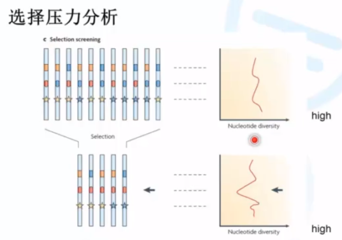
原始群体中，遗传多样性是十分高的，整个序列的核酸diversity都高。而在受到选择之后，diversity会发生波动。核酸多样性下降 可能就是由于under selection导致的。

在演化/驯化过程中，如果某一基因X占优势，即X的基因型占据主导地位，则基因X所在区域的杂合率/多样性会显著下降。本质就是 比较基因组不同区域多样性（杂合率）的变化

• 群体遗传关心的问题：
  • 遗传结构（phylogeny+structure）
  • 基因组上受选择区域：群体水平基因组不同位置的区域遗传多样性变化的规律（例如：Pi、Tajima’s D, Fst）
• 变异类型：
  • 中性突变（同义、相同类型的氨基酸、不影响环境适应性）：平衡选择，这种基因型频率是大致恒定的
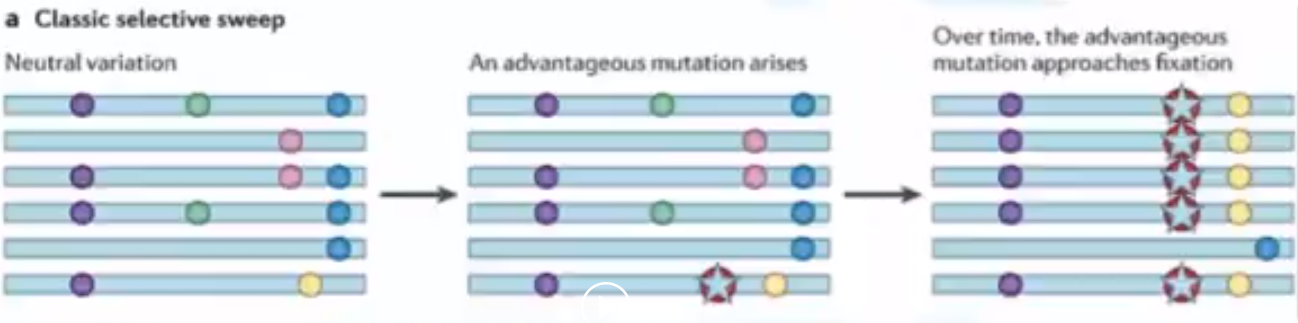
  • 有利突变（正选择）：选择扫荡（Selective sweep），与有利突变的中性突变的频率会显著提升
    
  • 有害突变（负选择）：背景选择（negative selection/background selection/ purifying selection） 是潜在的噪音

负选择会对正选择有一定的干扰作用，都能产生大量的低频突变，但是正选择会产生相对较多的高频突变。

两个亚群体之间的比较

多样性水平在亚群间比较，一般包括线性相关分析、亚群体间的差异比较两类。动植物重测序多是后者。Fst/pi ratio基于pi值。

1. 群体分化程度Fst (Fixation index): 比较两个亚群体间的Pi值和亚群体内的Pi值的差异。
   • 由PI值计算演变来（序列两两差异取均值）
   • 两个亚群体在某一段seq区域的差异度。0是无差异，数值越大，则说明两个亚群体之间已经发生了明显的分化（亚群内个体相似，亚群间差异大）

1

Fst=(\pi(between) - \pi(within))/ \pi(between)

2. 多样性变化倍数Pi ratio：某区间在亚群间的多样性差异的倍数，简单粗暴，就关注多样性值的高低变化。
   • 例如野生群体A/栽培群体B；野生群体A的多样性较高，而栽培群体B的多样性较低，所以多样性降低最显著的基因组区域，就与驯化改良基因相关
3. 其它比较值：ROD值、XP-CLR值等。而多个品种间的比较分化差异的di值

基于haplotype单体型的比较

前面pi/fst等都是基于SNP位点的多态性来检测潜在的选择信号区域。另一种方法是基于单体型haplotype的选择信号的检测。在selective sweeps选择过程中，有些强烈受到选择的位点variants由于LD的因素会连带着其附近的位点variants一起被保留，并且不会受到重组recombination的打断。一些低重组区域的haplotypes的长度会高于那些高重组区域的haplotypes的长度。因此，对比同一genomic区域在不同群体中的haplotype的长度可以用来判断是否受到选择。例如：在一个群体内部，如果某一个体强烈受到选择，其haplotype的长度会远长于其它个体；同理，对于两个群体之间的比较，某一群体受到选择，则其基因组中的受选择区域的haplotypes会比未受到选择群体中的haplotypes更长。

检测haplotype的选择信号最好利用定相phased后的数据集。方法有EHH和CLR法。这里利用R包中的rehh包进行分析。rehh有强大的说明和教程文档，后续深入了解其原理时值得进一步学习研究。rehh tutorial

rehh的实践

1. 读取数据。分别读取两个群体的phased的vcf数据
   • polarize_vcf设为FALSE. because we have not used an outgroup genome to set our alleles as derived or ancestral
   • 根据maf进行过滤位点

     1 2 3 4 5 6 7 8

     # read in data for each species# house house_hh <- data2haplohh(hap_file = "./house_chr8.vcf.gz",polarize_vcf = FALSE) # bactrianus bac_hh <- data2haplohh(hap_file = "./bac_chr8.vcf.gz",polarize_vcf = FALSE) ## filter on MAF - 0.05 house_scan <- scan_hh(house_hh_f, polarized = FALSE) bac_scan <- scan_hh(bac_hh_f, polarized = FALSE)

2. 计算计算单体型的iHS值。
   • polarized = FALSE
   • freqbin =1 if we know the ancestral allels or derived allels. rehh can apply weights to different bins of allele frequencies in order to test whether there is a significant deviation in the iHS statistic.
   • log Pvalue用于检测outliers值点，

     1 2 3 4 5 6 7 8 9 10

     ## perform haplotype genome scan- iHS house_scan <- scan_hh(house_hh_f, polarized = FALSE) bac_scan <- scan_hh(bac_hh_f, polarized = FALSE) ## perform iHS on house house_ihs <- ihh2ihs(house_scan, freqbin = 1) ### plot the iHS statistics ggplot(house_ihs$ihs, aes(POSITION, IHS)) + geom_point() ### plot the log P-value ggplot(house_ihs$ihs, aes(POSITION, LOGPVALUE)) + geom_point()

3. 计算群体之间的EHH值 xpEHH
   • 计算 cross-population 的 EHH test。利用之前iHS检测出的iES值。
   • include_freq=T,we get the frequencies of alleles in our output, which might be useful if we want to see how selection is acting on a particular position

     1 2 3 4 5 6

     ## perform xp-ehh house_bac <- ies2xpehh(bac_scan, house_scan, popname1 = "bactrianus", popname2 = "house", include_freq = T) #PLOT the xpEHH values ggplot(house_bac, aes(POSITION, XPEHH_bactrianus_house)) + geom_point()

     
     负数值代表在pop2(house in this case)中的强烈的选择信号。

4. 检测受选择区域中的haplotype structure

1
2
3
4
5
6
7
8
9
10
11
12
13
14
15

# find the highest hit 以最显著的位点做示例
hit <- house_bac %>% arrange(desc(LOGPVALUE)) %>% top_n(1)
# get SNP position
x <- hit$position # POSITION 19191935

# detect the position which the selection occured in the haplotype objects
marker_id_h <- which(house_hh_f@positions == x)
marker_id_b <- which(bac_hh_f@positions == x)

# calculate the bifurcation of haplotypes around our site of selection
house_furcation <- calc_furcation(house_hh_f, mrk = marker_id_h)
bac_furcation <- calc_furcation(bac_hh_f, mrk = marker_id_b)
# plot the bifurcation plot
plot(house_furcation, xlim = c(19.18E+6, 19.22E+6))
plot(bac_furcation, xlim = c(19.18E+6, 19.22E+6))

house_furcation

bac_furcation

1
2
3
4
5
6
7
8

# calculate the haplotype length around our signature of selection.
house_haplen <- calc_haplen(house_furcation)
bac_haplen <- calc_haplen(bac_furcation)

# see how haplotype structure differs between our two populations.

plot(house_haplen)
plot(bac_haplen)

house_furcation

bac_furcation

the blue haplotype is much larger around this target and is also more numerous in the European house sparrow.

5. 输出数据

1
2
3
4

# write out house bactrianus xpEHH
house_bac <- as_tibble(house_bac)
colnames(house_bac) <- tolower(colnames(house_bac))
write_tsv(house_bac, "./house_bac_xpEHH.tsv")

https://speciationgenomics.github.io/